AI Inventory Optimization
Forecasting accuracy does not necessarily translate into the lowest inventory cost.
A research study comparing 12 forecasting models across M5 and Store demand datasets — from traditional methods to neural approaches.
The central finding
Forecast quality and inventory economics can point to different winners.
Forecast quality
Inventory economics
The model that forecasts best does not necessarily produce the cheapest inventory decision.
LSTM wins on both forecast accuracy and inventory cost in this dataset.
At a glance
Key metrics
Research findings · frozen evidence · v1.0-evidence-freeze
Forecasts are the mechanism. Inventory is the outcome.
Forecasts are the mechanism. Inventory is the outcome. The frozen record of the study — the question, the data, the design, the models, and what the evidence actually shows.
01 · Research question
"How does the effectiveness of AI-based inventory optimization change as we move from traditional forecasting models toward neural-network approaches, when effectiveness is measured at the level of inventory outcomes rather than forecast errors alone?"
02 · Why this matters
Textbookforecast → accuracy
Realityforecast → inventory decision → cost · stockout · service
A forecast that is slightly less accurate can still produce the better inventory decision — and accuracy gains that do not change the decision may not be worth their cost.
03 · Experimental design
One common policy for every model: daily-review order-up-to with lost sales, L7 / 95% / H=1 / P=5.
04 · Models
Baselines: Naive · Seasonal Naive · Moving Average — Smoothing: SES · DES · TES — Statistical: ARIMA(1,1,0) · SARIMA (Store-only) — Intermittent: Croston · SBA · TSB (M5-only) — Neural: LSTM (global, one network per dataset). LLM: designed, not executed — no LLM number appears in the findings.
05 · Forecast evaluation
Primary: MASE — seasonal period 7. Secondary: MAE · RMSE · sMAPE · WAPE. 112,000 forecasts per model-dataset · 91 paired comparisons with Holm correction.
06 · Inventory simulation
Daily-review order-up-to policy with lost sales.
safety stock = z × σ_forecast × √L
Total cost = holding + stockout.
07 · Results
M5 (Intermittent demand) — Total Simulated Inventory Cost
Total cost · cost (H=1 units) · lower is better
Store Item Demand (Smooth demand) — Total Simulated Inventory Cost
Total cost · cost (H=1 units) · lower is better
| Dataset | Forecast winner · MASE | Inventory winner · cost | Policy wins |
|---|---|---|---|
| M5 | LSTM · MASE 1.316 | LSTM · cost 152.83 | 25 / 27 policies |
| Store | LSTM · MASE 0.978 | Moving Average · cost 2,084.50 vs LSTM 2,247.46 | Fragmented |
08 · The key finding
FORECAST ACCURACY ≠ INVENTORY COST
The winning model depends on the decision objective.
- A model can produce better forecasts while producing a worse inventory decision.
- The best forecasting model isn't necessarily the best inventory policy.
- Inventory performance depends on how forecast behavior interacts with the common policy — not on point accuracy alone.
09 · Limitations
- Smooth archetype n = 1.
- SARIMA Store-only. Croston family M5-only.
- Single policy family. H28 horizon.
Generalizability beyond these datasets and policy framework is not claimed.
10 · Conclusion
Forecasting performance should be evaluated through its operational consequences, not in isolation.
Model sophistication does not universally improve inventory outcomes.
The research question
Does forecasting sophistication improve inventory decisions?
How does the effectiveness of AI-based inventory optimization change from traditional forecasting models to large language model–based approaches?
A forecast is not the end of the story. It feeds a decision, and the decision produces the business outcome: forecast → inventory decision → cost, stockout, service level.
RQ1 — How do traditional, statistical, neural-network, and LLM-based approaches differ in demand forecasting performance?
RQ2 — How do forecasting differences translate into inventory-management outcomes?
RQ3 — Does increasing model sophistication consistently improve inventory performance?
RQ4 — Are model-performance patterns consistent across different retail demand environments?
RQ5 — What trade-offs exist between accuracy, inventory performance, computational requirements, and complexity?
Why inventory
Forecasting is the mechanism. Inventory is the outcome.
A successful forecast does not create business value by itself — the decision it enables does. Forecast quality is measured with MAE, RMSE, sMAPE, MASE on the same evaluation periods; inventory performance with total cost, holding, stockouts, service level, and average inventory, simulated under one common policy.
A forecast that is slightly less accurate can still produce the better inventory decision — and accuracy gains that do not change the decision may not be worth their cost.
Methodology
Twelve approaches, one ladder of increasing complexity
| Rung | Model | Family |
|---|---|---|
| 01 | Naive — Last observed value carried forward | Traditional |
| 02 | SNaive — Seasonal Naive — last week repeated | Traditional |
| 03 | MA — Moving Average | Traditional |
| 04 | SES — Simple Exponential Smoothing | Traditional |
| 05 | DES — Double Exponential Smoothing (Holt) | Traditional |
| 06 | TES — Triple Exponential Smoothing (Holt-Winters) | Traditional |
| 07 | ARIMA — Autoregressive Integrated Moving Average | Statistical |
| 08 | SARIMA — Seasonal ARIMA (Store-only by design) | Statistical |
| 09 | Croston — Intermittent-demand method (M5-only) | Statistical |
| 10 | SBA — Syntetos–Boylan Approximation (M5-only) | Statistical |
| 11 | TSB — Teunter–Syntetos–Babai (M5-only) | Statistical |
| 12 | LSTM — Long Short-Term Memory network | Neural |
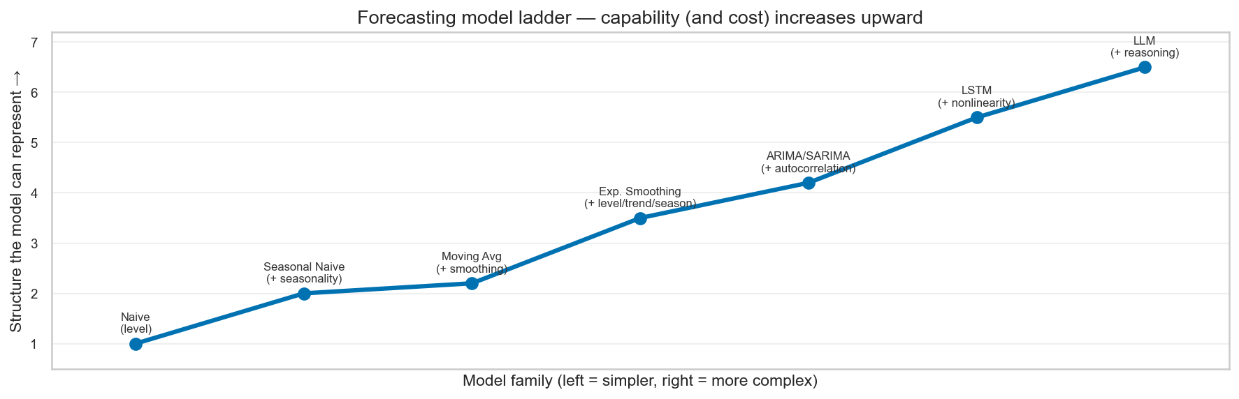
LLM is included as a design rung (see 11_src/llm_experiment_design.md); the LLM experimental phase was not executed, so no LLM result appears in the findings.
Walmart M5 — sparse and intermittent (64.5% zero rate). Store Item Demand — dense, nearly every item sells every day (0.02%). A method that performs well in one environment may perform poorly in the other, so every claim is tested in both: 500 series each, 8 rolling origins, 28-day horizon, seed 42.
Temporal split: train 2013-01-01 → 2015-10-31 (1,034 days) · validation 2015-11-01 → 2016-02-29 (121 days, incl. leap day) · test 2016-03-01 → 2016-05-22 (83 days). Common policy for all models: daily-review order-up-to with lost sales, L7 / 95% / H=1 / P=5.
Sensitivity grid · who wins
LSTM takes 25 of 27 policy cells — a robust winner.
Publication · September 2026 · Evidence freeze edb42ad
From Forecasts to Shelf Decisions
Evaluating AI-Based Inventory Optimization from Traditional Methods to Neural Forecasting. Read online in the Research reader or download the PDF.
Central thesis — frozen evidence
Forecast winner ≠ inventory winner
Forecasting accuracy does not necessarily translate into the lowest inventory cost.
LSTM wins forecast accuracy on both datasets (M5 MASE 1.316, Store MASE 0.978). Moving Average wins Store inventory cost (2,084.50 vs LSTM 2,247.46) under the default policy.
Frozen published evidence · tag v1.0-evidence-freeze. Interrogate it in the Lab; read it in the research reader.
Want to test the result?
Explore the Lab →